A Finite Element mesh is the discretization of a continuous geometry into finite parts (elements).
An FE solver calculates the displacements at individual nodes of the elements. We are also interested in what happens in the volume (or area for 2-D elements) of the element. But this information is not directly available from the nodal results.
The displacements for the regions between the nodes are interpolated using equations called shape functions. The various element types differ in what shape functions they utilize for the interpolation.
The figure below shows the variations of a field variable (a quantity that varies continuously within an element – for example, displacement or temperature) within a 2-node line element [1]:

The exact solution may be modeled as linear or quadratic approximations. If the mesh is refined (imagine the distance, X between nodes 1 and 2 reducing) the modeled solution should converge with the exact solution (within some tolerance). Note that the linear approximation would require a more refined mesh than the quadratic approximation to match the exact solution.
Shape function are the mathematical expressions that define these approximations. The shape function corresponding to the linear approximation is shown below [2]. N1 represents the situation where the maximum and minimum values of the field variables occur at Node 1 and Node 2 respectively.

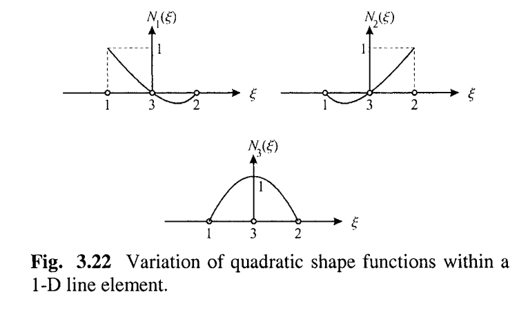
A quadratic shape function is shown below [3]:

You can read more about shape functions in the ANSYS theory manual.
Here is another post discussing the underlying theory of structural Finite Element Analysis.
References
[1] The Finite Element Method and Applications using ANSYS – Edrogan Madenci, Ibrahim Guven