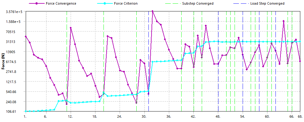
The figure below shows a force convergence plot from an ANSYS Workbench Mechanical run:

The X-axis shows the cumulative iteration number and the Y-axis shows the force in Newtons. A number of things can be said about this plot. Below, I will make a few comments in order to explain this plot and also clear up some confusions which some ANSYS users have regarding this plot and how it relates to the analysis and solution types.
This plot is only relevant for a Non-Linear Analysis
The underlying equation for structural FEA is [K]{U} = {F}
Where {F} is the input load vector and [K] is the global stiffness matrix. {U} is the unknown displacement vector which is solved for at each node in the model. In a linear analysis the global stiffness matrix is calculated only once.
There are three sources of non-linearities in an analysis : Material, Geometry (Large deformations) and contact iterations. If none of these are present in the analysis, then the analysis is linear.
In a Non-Linear analysis the global stiffness matrix is calculated at every iteration. In the above plot there are 68 equilibrium iterations. This means that the global stiffness matrix was formulated 68 times.
This plot is a visual representation of the progression of the Newton-Raphson method
The Newton-Raphson is a numerical technique used to solve a system of equations through an iterative process. Here is a step by step description of how it applies to Non-Linear structural analysis:
- Consider the equation [K]{U} = {F}. The objective is to determine {U} for a given {F} which is the applied load
- Start with zero initial displacements, {U}i = 0 and the applied load {F}
- Estimate the initial stiffness matrix [K]i – This stiffness matrix will be close to what would be calculated for a linear analysis.
- Determine {U}1 based on {F} and [K]i
- Calculate the global stiffness matrix [K]1 based on {U}1 and other non-linearities.
- Calculate the internal forces {F}1 based on [K]1 and {U}1
- Determine the residual forces {F}res = {F} – {F}1
- If {F}res is close to zero the solution has converged. This means that we have determined the displacements {U} (with sufficient accuracy) for the applied {F}
- If {F}res is not close to zero, then recalculate the displacements {U}2 based on {F} and {K}1
- Repeat steps 4 to 8 until the solution is converged.
It should be noted that it is step 5, i.e. the recalculation of the stiffness matrix which makes the internal forces different from the external (applied) forces.
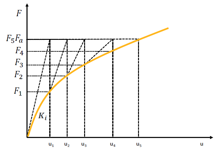
The figure below shows a graphical representation of the Newton-Raphson Method.

You may refer to this ANSYS training course which explains this process in details:
The above plot shows that convergence was achieved after 5 equilibrium iterations. In the force convergence plot from the ANSYS run, the first load step converged after 11 equilibrium iterations.
The Force-Convergence plot is not a representation of the solver type (Direct vs Iterative)
A common source of confusion arises from the use of the word “iterative”. The Newton-Raphson technique is an iterative process and there is a solver type which is iterative. “Iterative” refers to two different things.
In other words, the Newton-Raphson method is applied to Non-Linear analyses irrespective of the selected solver type.
What is the difference between direct and iterative solvers and what iterations are we talking about here?
So far we have discussed:
- In a linear analysis, the stiffness matrix [K] is calculated only once
- The matrix equation {F} = [K]{U} is solved only once
- In a non-linear analysis the stiffness matrix is evaluated multiple times
- Each evaluation of the stiffness matrix constitutes an equilibrium iteration
We can now add:
- Solver types have to do with the mathematical techniques on how to treat the stiffness matrix
- In a direct solver, the global stiffness matrix is converted to a sparse matrix by utilizing the sparseness of the stiffness matrix (i.e. zero terms). There is one matrix solver iteration per equilibrium iteration.
- An iterative solver takes multiple iterations to solve the equation [K]{U} = {F} once. There are multiple solver iterations per equilibrium iteration. The solver equations are internal to the ANSYS program and we do not see it represented in the solution output, or the force-convergence plot.
When we refer to an iteration we should be clear if we are referring to a matrix solve iteration (depends on the solver type) or an equilibrium iteration (depends on linear vs Non-Linear analysis).
Detailed information on direct and iterative solvers as used in ANSYS can be found here: https://www.mm.bme.hu/~gyebro/files/ans_help_v182/ans_thry/thy_tool8.html
Summary
The table below summarizes what we have discussed in this article:
| Solver Type | Analysis Type | Matrix Solver Iterations | Equilibriums Iterations |
| Direct | Linear | 1 | 1 |
| Direct | Non-Linear | 1 | ≥ 1 |
| Iterative | Linear | ≥ 1 | 1 |
| Iterative | Non-Linear | ≥ 1 | ≥ 1 |
It is worth noting that the direct solvers are more robust than iterative solvers (but more resource intensive). And solutions to linear analyses are more easy to obtain than those for non-linear analyses. Compare this to the number of iterations required for each analysis type and it makes sense that the more the iterations, the less robust the analysis is.
