Introduction

We recently discussed several methods of performing seismic analysis to determine the physical response of structures (Performing a Seismic Analysis – Four methods explained). We explained how some of the most robust numerical methods related to seismic analyses revolve around Response Spectra Plots . If you are not familiar with response spectra I would recommend that you take a look at the article referenced above.

In this article we will:

• Briefly go over the fundamental math behind seismic analysis
• Discuss the numerical technique used to calculate the response of structures
• Explain the logic (programming methodology) employed to obtain the numerical solution
• Generate the Response Spectrum Plot for the ground acceleration data for El Centro 1940 Earthquake and compare the results to published literature.

The Fundamental Math behind Seismic Analysis

When we say “fundamental” we imply the governing equations which are used to describe the response of structures exposed to seismic activity. We will briefly mention the equations that are relevant to our analysis.

Consider a linear single degree of freedom system (SDOF) with :

Mass, m
Stiffness, k
and a time varying force, P(t)

The equation of motion describing the behavior of this system is given by:

where,

u is displacement
u’ is velocity
u” is acceleration
and c is the viscous damping coefficient

If a structure was approximated as a SDOF the above equation could be used to estimate its response. As long as we have values for m, k and c, we could determine the response of the structure (displacement, acceleration or velocity) to a given excitation, P(t). Textbooks on numerical analysis and system dynamics cover the solution process for this equation in detail. As an example, you may study chapter 5 (Numerical Evaluation of Dynamic Response) of Dynamics of Structures fourth Edition by Anil Chopra.

In many cases however, we do not know the mass or stiffness of a structure and are not in a position to readily make reasonable assumptions. In these situations it is helpful to consider an alternative form of equation 1. By dividing equation 1 by m and utilizing the fact that angular frequency,

we can come up with the following form of the equation of motion:

where ζ is the damping ratio, or fraction of critical damping and is given by

Equation 2 is written adapted to seismic analysis where the subscript g refers to ground (u”g (t) is ground acceleration) and n is for natural frequency. Let this equation sink in for a bit… this result is extremely powerful!

It can be seen that for a given u”g(t), the deformation response u(t) of the system depends only on the natural frequency ωn or natural time period Tn of the system and its damping ratio, ζ ; writing formally, u ≡ u(t, Tn, ζ).

Thus any two systems having the same values of Tn and ζ will have the same deformation response u(t) regardless of how they may differ in mass and stiffness.

Central Difference Method

Several numerical techniques may be utilized to solve equation 2. The method that we will present here is the Central Difference Method. This method is based on a finite difference approximation of the time derivatives of displacement (velocity and acceleration). Taking a constant time increment delta T, the central difference velocity and accelerations may be represented as:

where the subscript i represents the ith time step.

The expression for u’i is self explanatory. It can be seen that u”i is also expressed in terms of the displacements (rather than the velocity). You can view the derivation for these two expressions in this video: Central Difference Method at around the 3:30 mark.

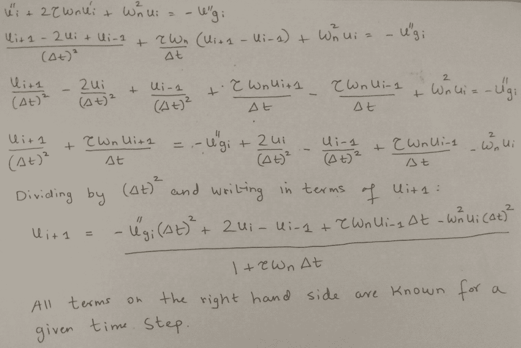
The heart of the central difference method lies in substituting the above expressions for velocity and expression into the equation of interest (in our case equation 2) and stating the equation in terms of ui+1. When evaluating ui+1, the values of ui and ui-1 will be known from the implementation of the procedure for the previous time steps (or the boundary condition for the first step).

For a system initially at rest (as is typical for structures exposed to seismic loading) u(0) = 0

Below is my derivation for the expression for ui+1 in terms of the known terms starting from Equation 3 and the central difference expressions above.

Programming the Central Difference Method to achieve a numerical solution

Below is an excerpt from an excel spreadsheet where I programmed the central difference method. The iterations happen under the “displacement iterations” cells.

The logic goes like this:

• Ui(0) = 0

• Ui-1 is equal to the value of Ui in the previous cell – The yellow Ui-1 cell value is taken from the yellow Ui cell and the process repeated for all cells
• Ui is equal to the value of Ui+1 in the previous cell – The green Ui cell value is taken from the green Ui+1 cell and the process repeated for all cells
• Ui+1 is equal to the expression derived above
• The iterative process solves for the displacement response. The velocity and acceleration responses can be calculated using the central difference method

My excel program does not loop over the input values for frequency and damping. I developed a code in python for that purpose.

Generating a Response Spectrum Curve with Python – Studying the El Centro 1940 Earthquake

The El Centro earthquake of 1940 is one of the most studied real world excitation within earthquake engineering.

USGS Description of the El Centro (Imperial Valley) Earthquake:
Nine people were killed by the May 1940 Imperial Valley earthquake. At Imperial, 80 percent of the buildings were damaged to some degree. In the business district of Brawley, all structures were damaged, and about 50 percent had to be condemned. The shock caused 40 miles of surface faulting on the Imperial Fault, part of the San Andreas system in southern California. It was the first strong test of public schools designed to be earthquake-resistive after the 1933 Long Beach quake. Fifteen such public schools in the area had no apparent damage. Total damage has been estimated at about $6 million. The magnitude was 7.1. [1]

The ground acceleration data for El Centro 1940 is available, and was used to verify the python code. The ground acceleration is in the North-South direction as shown below:

The image below shows the displacement response for this data set:

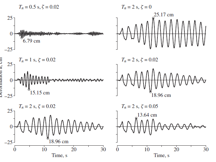
For comparison purposes, the top left (Tn=0.5 s, Zeta=0.02) and bottom right (Tn=2 s, Zeta = 0.05) systems were analyzed with Python. The plots are shown below and are in good agreement with the published data.

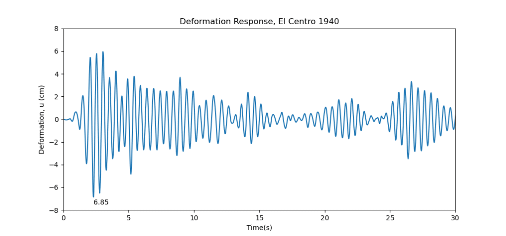
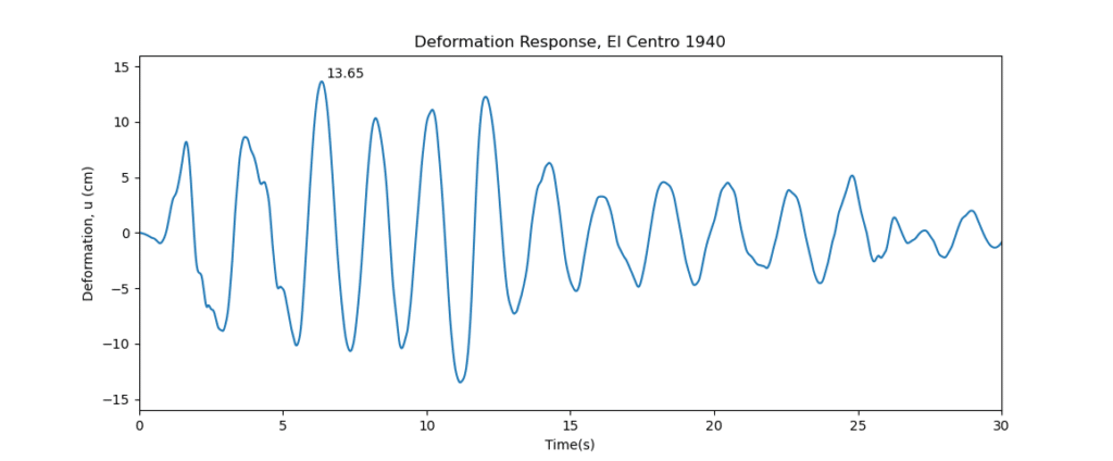
These are deformation responses. Similar plots can be plotted for velocity and acceleration.

In order to generate a response spectrum we have to:

• Obtain plots similar to the ones above for a range of time periods (and critical damping coefficients)
• Keep track of the maximum absolute response
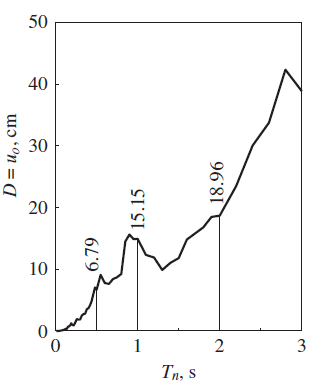
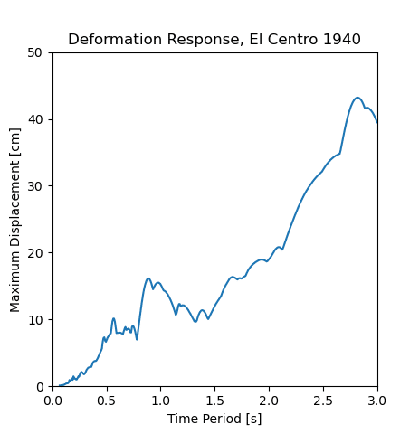
• Generate a plot of the time period vs the maximum response for that time period

Figure 7 shows the displacement response spectrum as published in ref [2]. Figure 8 shows the response curve generated by the python program. The two plots agree barring potentially some discretization errors causing slight discrepancies. Figure 8 was generated for 400 points between 0 and 3 s.

Response Spectrum with Spectral Acceleration

The maximum deformation of the SDOF is one way of representing an excitation. There are several other methods, some being especially useful in earthquake engineering.

Consider a quantity A for a SDOF system with natural frequency ωn related to its peak deformation D ≡ uo due to earthquake ground motion:

The quantity A has units of acceleration and is related to the peak value of base shear Vb [or the peak value of the equivalent static force, Feq]:

Vb = Feq = mA

The response spectrum plot for A is shown in Figure 9 below. Figure 10 shows the same plot generated via Python code.

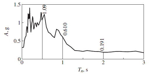
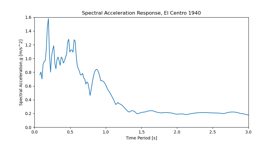
A Pseudo-Response Spectrum plot can be used to determine the equivalent static load for a structure exposed to seismic loads. The value of A corresponding to the natural frequency of a structure can be applied in a static structural analysis to determine its response. A modal analysis along with a value for the dynamic amplification factor would typically be needed for this purpose.

References

[1] https://www.vibrationdata.com/elcentro.htm
[2] Chopra, Dynamics of Structures 4th Ed