Contact interactions play a pivotal role in ensuring realistic results in structural simulations involving assemblies. Whether it’s load transfer across bolted joints, pressure in gasket interfaces, or friction between sliding parts, properly defined contact behavior is essential. Ansys Workbench offers a powerful utility—the Contact Tool—for both diagnosing contact setup and evaluating contact performance during or after simulation. This guide provides a complete walkthrough of its capabilities, setup methods, and best practices.
What Is the Contact Tool?
The Contact Tool is a built-in analysis object in Ansys Workbench that allows you to:
- Evaluate initial contact conditions (before solving)
- Diagnose contact behavior as part of a solved result
- Verify whether contacts are transferring loads as expected
- Examine and group contact results using a unified scoping
It can be inserted under:
- The Connections branch (for pre-solution checks),
- The Solution branch (for post-solution analysis), or
- The Solution Combination branch (limited to pressure, frictional stress, penetration, and gap).
When to Use the Contact Tool
The Contact Tool is especially useful when:
✅ You’re unsure whether contact pairs are correctly defined or engaged
✅ You want to verify if parts are bonded, sliding, or separating during load
✅ Solver convergence issues suggest contact nonlinearity or unrealistic stiffness
✅ You need to post-process results like contact pressure or frictional stress
✅ You want to evaluate initial gaps, penetration, or status before solving
Scoping Methods: Worksheet vs. Geometry Selection
The Contact Tool supports two scoping approaches:
🔹 Worksheet Method
- Scope is defined by selecting specific contact regions.
- Best for precise evaluation of known contact pairs.
- Enables evaluation of Initial Information (pre-solution status).
- Allows sorting by contact type (Bonded, Frictional, etc.) and behavior (linear/nonlinear).
🔹 Geometry Selection Method
- Scope is defined by selecting model geometry (e.g., bodies or faces).
- Useful when you want to evaluate all contacts associated with certain parts / faces.
- Cannot be used for initial contact evaluations—only post-solution.
Evaluating Initial Contact Conditions (Pre-Solution)
To check contact status before solving:
- Insert the Contact Tool under the Connections branch.
- Choose Worksheet in the Scoping Method field (default).
- Select contact regions via:
- Manual checkbox selection,
- Copy-paste from the Connections branch,
- Drag-and-drop of groups (e.g., All Contacts, Nonlinear Contacts).
- Right-click and choose Generate Initial Contact Results.
- Review the Initial Information table.
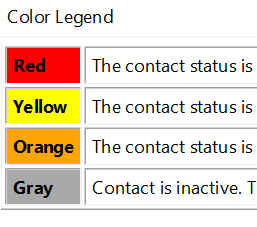
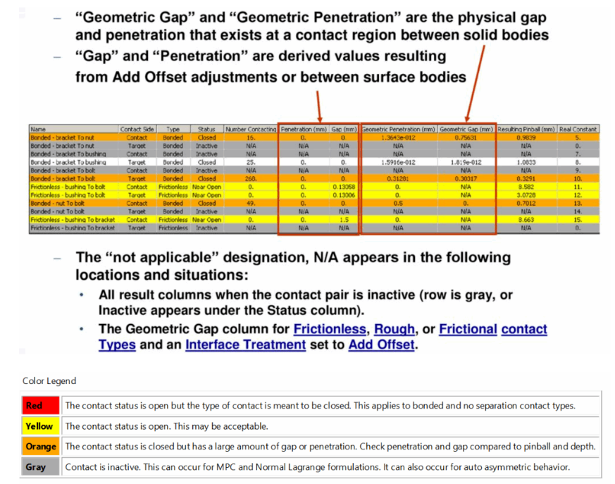
🔍 Color-Coded Status (Initial Contact)
| Color | Meaning |
|---|---|
| Red | Contact is open, but should be closed (e.g., bonded/no separation). Likely setup error. |
| Yellow | Open contact—acceptable for nonlinear types (frictional, rough, etc.). |
| Orange | Contact is closed but with large gap or penetration. May cause stiffness or convergence issues. |
| Gray | Contact is inactive (due to MPC, Lagrange, or auto-asymmetric behavior). |
The tool assumes small deflection for initial evaluation, which affects calculations like the Pinball Radius. The image shows an illustration of the contact tool.
Evaluating Contact Behavior (Post-Solution)
To inspect contacts after solving:
- Insert the Contact Tool under the Solution branch.
- Choose either Worksheet or Geometry Selection for scoping.
- Worksheet : Solution –> Insert –> Contact Tool –> Contact Tool
- Geometry Selection : Solution –> Select faces or bodies –> Right click –> Insert –> Contact Tool –> Contact Tool
- Add desired result types: Right click Contact Tool –> Insert ( Status, Pressure, Gap, Penetration, Frictional Stress etc.).
- Solve or update the solution branch.
- View contact plots and data in the Results tab.
🧾 Common Results
| Result | What It Shows |
|---|---|
| Contact Status | Open/Closed/Sticking/Sliding status under applied load |
| Contact Pressure | Normal force transferred at the interface |
| Penetration | Overclosure between contact and target surfaces |
| Gap | Separation distance in open or unloaded areas |
| Frictional Stress | Shear stress from sliding or attempted slip between contact faces |
These can be plotted across multiple regions at once when scoped through a single Contact Tool.
Practical Tips
- Refine mesh in contact regions
Use face or body sizing to ensure smaller elements at contact interfaces. This improves accuracy and reduces artificial penetration.
- Ensure mesh compatibility for bonded and no-separation contacts
Apply matching mesh controls (e.g., face sizing or mapped meshing) on both sides, or use shared topology during geometry prep to align nodes.
- Enable contact diagnostics early in nonlinear simulations
Insert a Contact Tool under the Solution branch and add Status, Pressure, Penetration, and Frictional Stress results to catch issues during test runs.
- Use staggered loading to allow progressive engagement
Ramp loads gradually using multiple load steps or tabular definitions. Enable large deflection and automatic time stepping for stability.
- Run Initial Information checks before solving
Insert the Contact Tool under the Connections branch and generate Initial Contact Results to detect gaps or invalid contact setups.
- Compare penetration to pinball radius or contact depth
Excessive penetration (typically >50% of pinball radius) signals poor mesh or stiffness. Adjust geometry or refine the mesh accordingly.
Limitations and Caveats
- Initial contact evaluation only works with the Worksheet Method.
- In the Solution Combination branch, only a subset of results is available.
- If contacts share elements across conditions (e.g., multiple contact pairs involving the same surface or body region), the Contact Tool aggregates data—use User Defined Results with Element Type IDs to isolate results for a specific contact pair.
- Results for far-field elements outside the pinball region are not written to the
.rstfile (to save space).
Conclusion
The Contact Tool in Ansys Workbench is not just a diagnostic add-on—it’s essential for verifying physical realism in contact-based simulations. From validating bonded connections to debugging frictional slip or solver divergence, it helps you take control of one of the trickiest parts of FEA modeling.
References
[1] Ansys Training Material : https://slideplayer.com/slide/14150938/